精度详解与实践

📄 各精度类型介绍
📑 混合精度理解
- 📑 Mixed Precision Training
- 📄 使用混合精度对大语言模型进行加速

❓ 问题导航

有哪些精度？如何理解每个精度的计算方式？
- 各精度类型介绍¹
混合精度计算流程是什么？怎么从代码实现？
- 通常使用 Pytorch 的 autocast context manager 和开源的 Fabric Pypi 进行混合精度的计算，很方便，详细参考: A Mixed-Precision Code Example²。
为什么要用混合精度？
- 对于 memory-limited 算子， Fp16 相对于 Fp32 可以减小一半的访存，能提升算子性能
- 减小模型显存占用，相同条件下，可以使用更大的 batch size，或者是更复杂的模型
- 对于计算密集的算子，比如 linear， conv 等通过 Tensor Cores 可以进行加速
- FP64 到 FP32（单精度），对模型计算影响不大。但是 FP32 到 FP16 会出现 Overflow 和 Underflow 的情况，所以需要用混合精度去平衡计算速度（采用 16bit）、Overflow（解决方案：bfp16 or fp32）、Underflow（解决方案：fp16 or fp32）。详细参考：From 32-Bit to 16-Bit Precision³
- 采用了 FP16 和 FP32 混合精度的模型质量，比单纯全 FP32 的的模型，推理准确度更高。这是因为，当采用 FP16 降低精度的时候，引入了一些燥声，这些燥声对防止训练的过拟合具有一定作用（over-fit），如下图，模型为 DistilBert，66M 参数量。
- 主要注意的是 bfloat16 的 10 进制间隔精度是 0.01（注：在-1～1 之间精度是 0.001），表示范围是[-3.40282e+38，3.40282e+38]。可以明显的看到 bfloat16 比 float16 精度降低了，但是表示的范围更大了，能够有效的防止在训练过程中的溢出。
大模型中不同精度占用的显存大小？(参考上图，DistilBert 模型（66M 参数量） Memory allocated)
- 混合精度理解⁴
模型训练中的各 weight、gradients 的 scale 是怎么转换的？

探索 TO DO

FP8 的看法：
1. 用 FP8 训练大模型有多香？微软：比 BF16 快 64%，省 42% 内存
  
  https://www.jiqizhixin.com/articles/2023-11-02-10
2. 题外话，前不久去 X 公司跟 X 总监聊下一代 AI 芯片架构的时候，他认为下一代芯片可以不需要加入 INT8 数据类型，因为 Transformer 结构目前有大一统 NLP 和 CV 等领域的趋势，从设计、流片到量产，2 年后预计 Transformer 会取代 CNN 成为最流行的架构。我倒是不同意这个观点，目前来看神经网络的 4 个主要的结构 MLP、CNN、RNN、Transformer 都有其对应的使用场景，并没有因为某一种结构的出现而推翻以前的结构。只能说根据使用场景的侧重点比例有所不同，我理解 Int8、fp16、fp32 的数据类型在 AI 芯片中仍然会长期存在，针对不同的应用场景和计算单元会有不同的比例。

‍

各精度类型介绍

https://zhuanlan.zhihu.com/p/657886517

FP16

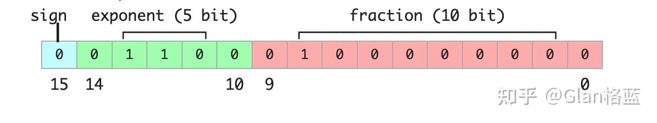
FP16 也叫做 float16，两种叫法是完全一样的，全称是 Half-precision floating-point(半精度浮点数)，在 IEEE 754 标准中是叫做 binary16，简单来说是用 16 位二进制来表示的浮点数，来看一下是怎么表示的(以下图都来源于维基百科 ^[2]^)：

其中：
- Sign(符号位): 1 位，0 表示整数；1 表示负数。
- Exponent(指数位)：5 位，简单地来说就是表示整数部分，范围为 00001(1)到 11110(30)，正常来说整数范围就是** ** ，但其实为了指数位能够表示负数，引入了一个偏置值，偏置值是一个固定的数，它被加到实际的指数上，在二进制 16 位浮点数中，偏置值是 15。这个偏置值确保了指数位可以表示从-14 到 +15 的范围即** ** ，而不是 1 到 30，注：当指数位都为 00000 和 11111 时，它表示的是一种特殊情况，在 IEEE 754 标准中叫做非规范化情况，后面可以看到这种特殊情况怎么表示的。
- Fraction(尾数位)：10 位，简单地来说就是表示小数部分，存储的尾数位数为 10 位，但其隐含了首位的 1，实际的尾数精度为 11 位，这里的隐含位可能有点难以理解，简单通俗来说，假设尾数部分为 1001000000，为默认在其前面加一个 1，最后变成 1.1001000000 然后换成 10 进制就是:** **
```
# 第一种计算方式
1.1001000000 = 1 * 2^0 + 1 * 2^(-1) + 0 * 2^(-2) + 0 * 2^(-3) + 1 * 2^(-4) + 0 * 2^(-5) + 0 * 2^(-6) + 0 * 2^(-7) + 0 * 2^(-8) + 0 * 2^(-9) = 1.5625
# 第二种计算方式
1.1001000000 = 1 + 576(1001000000变成10进制)/1024 = 1.5625
```
所以正常情况下计算公式就是：

\begin{aligned} & (-1)^{\text {sign }} \times 2^{\text {exponent-15 }} \times 1 . \text { fraction }(2 \text { 进制 }) \\ & (-1)^{\text {sign }} \times 2^{\text {exponent-15 }} \times\left(1+\frac{\text { fraction }(10 \text { 进制 })}{1024}\right)\end{aligned}

‍

举一个例子来计算，这个是 FP16(float16)能表示的最大的正数：

$0111101111111111=(-1)^0 \times 2^{30-15} \times\left(1+\frac{1023}{1024}\right)=65504$

同样，这个是 FP16(float16)能表示的最大的负数：

$1111101111111111=(-1)^1 \times 2^{30-15} \times\left(1+\frac{1023}{1024}\right)= -65504$

这就是 FP16(float16)表示的范围[-65504，65504]。

我们来看一些特殊情况，FP16(float16)能表示最小的正数是多少呢？

$0000000000000001=(-1)^0 \times 2^{1-15} \times\left(1+\frac{1}{1024}\right) \approx 0.000000059604645$

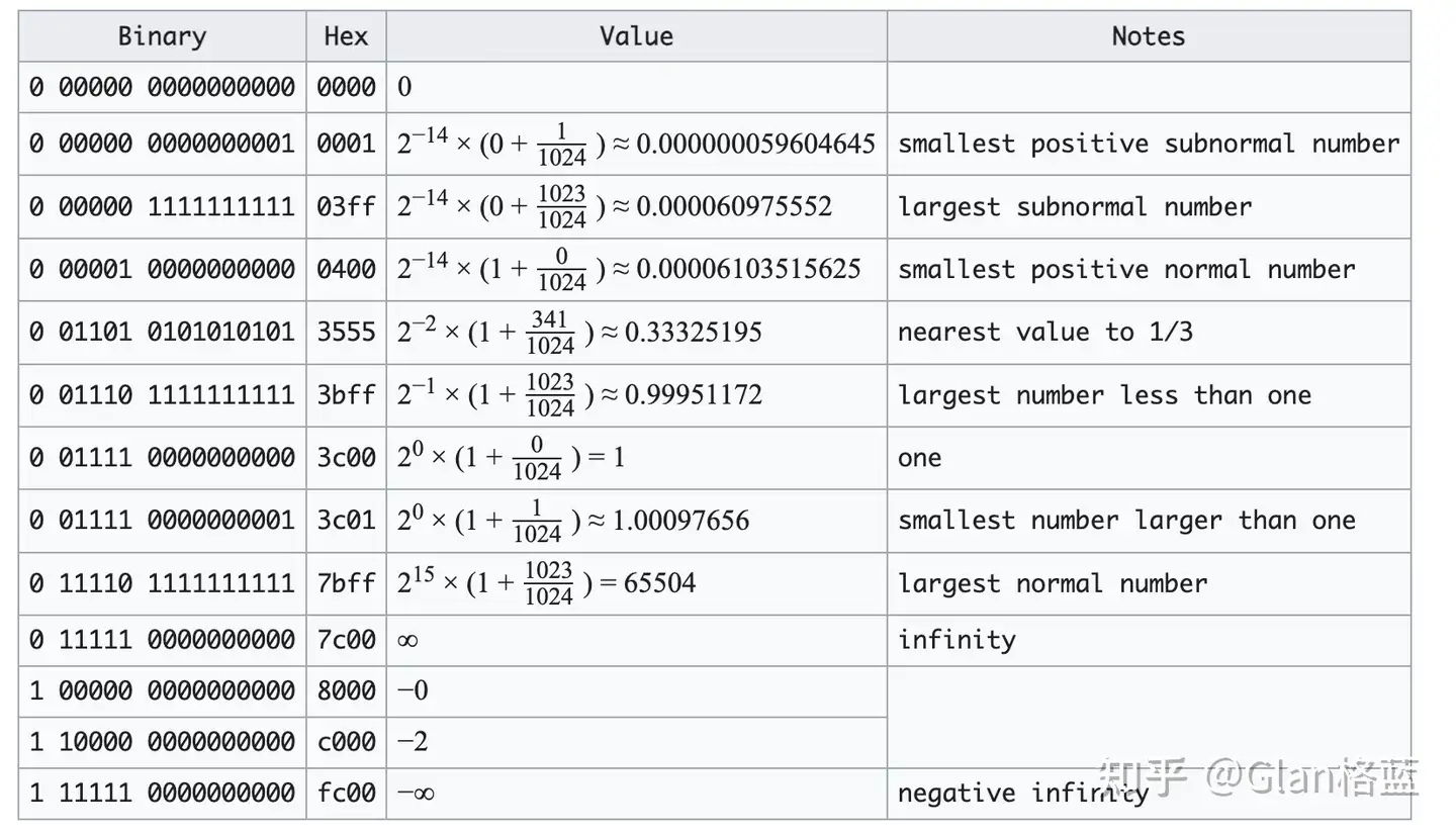
我们就不一一的计算了，贴一个 FP16(float16)特殊数值的情况：

上表中，subnormal number 是指指数位为全 0 的特殊情况情况，其他的也是一些常见的特殊情况。

接下来看一下在 pytorch 中是如何表示的：
```
torch.finfo(torch.float16)
# 结果
finfo(resolution=0.001, min=-65504, max=65504, eps=0.000976562, smallest_normal=6.10352e-05, tiny=6.10352e-05, dtype=float16)
```
一些解释：
1. resolution（分辨率）：这个浮点数类型的在十进制上的分辨率，表示两个不同值之间的最小间隔。对于** **torch.float16** ，分辨率是 0.001，就是说两个不同的 **torch.float16 数值之间的最小间隔是 0.001。
2. min（最小值）：对于** **torch.float16，最小值是 -65504。
3. max（最大值）：对于** **torch.float16，最大值是 65504。
4. eps（机器精度）：机器精度表示在给定数据类型下，比 1 大的最小浮点数，对于** **torch.float16，机器精度是 0.000976562，对应上表中的 smallest number larger than one。
5. smallest_normal（最小正规数）：最小正规数是大于零的最小浮点数，对于** **torch.float16，最小正规数是 6.10352e-05，对应上表中的 smallest positive normal number
6. tiny（最小非零数）：最小非零数是大于零的最小浮点数，对于** **torch.float16，最小非零数也是 6.10352e-05，也是对应上表中的 smallest positive normal number
这里要详细的解释一下 resolution（分辨率），这个是我们以十进制来说的两个数之间的最小间隔，我们看一个例子就会明白：
```
import torch

# 把10进制数转化为 torch.float16
num = 3.141
num_fp16 = torch.tensor(num).half()
print(num_fp16)
# 结果
tensor(3.1406, dtype=torch.float16)

num = 3.1415
num_fp16 = torch.tensor(num).half()
print(num_fp16)
# 结果
tensor(3.1406, dtype=torch.float16)
# 可以看到3.141和3.1415间隔只有0.0005，所以在float16下结果是一样的

num = 3.142
num_fp16 = torch.tensor(num).half()
print(num_fp16)
# 结果
tensor(3.1426, dtype=torch.float16)
# 可以看到结果不一样了
```
从上面代码可以看到，十进制中相隔 0.001，在 float16 中才会有变化，这个时候会有一个疑问，难道精度只有小数点后三位？那怎么之前见了很多参数都是有很多小数点的？那我们来看一下全过程，把 float16 变成 2 进制，再把 2 进制变成 16 进制：
```
import struct
def float16_to_bin(num):
    # 将float16数打包为2字节16位，使用struct.pack
    packed_num = struct.pack('e', num)

    # 解包打包后的字节以获取整数表示
    int_value = struct.unpack('H', packed_num)[0]

    # 将整数表示转换为二进制
    binary_representation = bin(int_value)[2:].zfill(16)
    return binary_representation

num = 3.141
num_fp16 = torch.tensor(num).half()
print(num_fp16)
binary_representation = float16_to_bin(num_fp16)
print(binary_representation)  # 打印二进制表示
# 结果
tensor(3.1406, dtype=torch.float16)
0100001001001000


num = 3.1415
num_fp16 = torch.tensor(num).half()
binary_representation = float16_to_bin(num_fp16)
print(binary_representation)  # 打印二进制表示
# 结果
tensor(3.1406, dtype=torch.float16)
0100001001001000  # 还是一样的结果

num = 3.142
num_fp16 = torch.tensor(num).half()
print(num_fp16)
binary_representation = float16_to_bin(num_fp16)
print(binary_representation)  # 打印二进制表示
# 结果
tensor(3.1426, dtype=torch.float16)
0100001001001001  # 不一样了
```
再看一下把 2 进制变成 16 进制：
```
def binary_to_float16(binary_string):
    # 检查输入是否是有效的16位二进制字符串
    if len(binary_string) != 16:
        raise ValueError("输入的二进制字符串必须是16位长")

    # 提取组成部分：符号、指数、尾数
    sign = int(binary_string[0])  # 符号位
    exponent = int(binary_string[1:6], 2)  # 指数位
    mantissa = int(binary_string[6:], 2) / 1024.0  # 尾数位，除以2的10次方（即1024）以获得10位精度

    # 根据符号、指数和尾数计算float16值
    value = (-1) ** sign * (1 + mantissa) * 2 ** (exponent - 15)
    return value

# 10进制3.141对应float16：3.1406
binary_representation = "0100001001001000"
# 将二进制表示转换为float16
float16_value = binary_to_float16(binary_representation)
print("通过2进制转化后Float16值:", float16_value)
# 结果：
通过2进制转化后Float16值: 3.140625

# 10进制3.1415对应float16：3.1406
binary_representation = "0100001001001000"
# 将二进制表示转换为float16
float16_value = binary_to_float16(binary_representation)
print("通过2进制转化后Float16值:", float16_value)
# 结果：
通过2进制转化后Float16值: 3.140625

# 10进制3.142对应float16：3.1426
binary_representation = "0100001001001001"
# 将二进制表示转换为float16
float16_value = binary_to_float16(binary_representation)
print("通过2进制转化后Float16值:", float16_value)
# 结果：
通过2进制转化后Float16值: 3.142578125
```
因为在计算机中是以 2 进制存储计算的，所以转换后的 float16 值会有很多位小数，但这些后面的小数是没有精度的，换成 10 进制的精度是只有 0.001 的。注：在-1~1 之间精度是 0.0001，因为有隐含位 1 的关系，大家可以试一下。

BF16

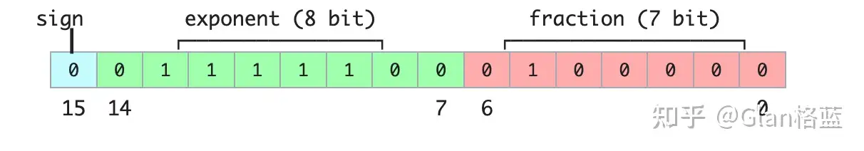
BF16 也叫做 bfloat16(这是最常叫法)，其实叫“BF16”不知道是否准确，全称 brain floating point，也是用 16 位二进制来表示的，是由 Google Brain 开发的，所以这个 brain 应该是 Google Brain 的第二个单词。和上述 FP16 不一样的地方就是指数位和尾数位不一样，看图：
- Sign(符号位): 1 位，0 表示整数；1 表示负数
- Exponent(指数位)：8 位，表示整数部分，偏置值是 127
- Fraction(尾数位)：7 位，表示小数部分，也是隐含了首位的 1，实际的尾数精度为 8 位
计算公式：

(-1)^{\text {sign }} \times 2^{\text {exponent-127 }} \times 1. fraction (2 进制 )

这里要注意一下，并不是所有的硬件都支持 bfloat16，因为它是一个比较新的数据类型，在 NVIDIA GPU 上，只有 Ampere 架构以及之后的 GPU 才支持，如何判断呢？很简单：
```
import transformers
transformers.utils.import_utils.is_torch_bf16_gpu_available()
# 结果为True就是支持
```
看一下在 pytorch 中是如何表示的：
```
import torch
torch.finfo(torch.bfloat16)
# 结果
finfo(resolution=0.01, min=-3.38953e+38, max=3.38953e+38, eps=0.0078125, smallest_normal=1.17549e-38, tiny=1.17549e-38, dtype=bfloat16)
```
主要注意的是 bfloat16 的 10 进制间隔精度是 0.01（注：在-1～1 之间精度是 0.001），表示范围是[-3.40282e+38，3.40282e+38]。可以明显的看到 bfloat16 比 float16 精度降低了，但是表示的范围更大了，能够有效的防止在训练过程中的溢出。

FP32

FP32 也叫做 float32，两种叫法是完全一样的，全称是 Single-precision floating-point(单精度浮点数)，在 IEEE 754 标准中是叫做 binary32，简单来说是用 32 位二进制来表示的浮点数，看图：
- Sign(符号位): 1 位，0 表示整数；1 表示负数
- Exponent(指数位)：8 位，表示整数部分，偏置值是 127
- Fraction(尾数位)：23 位，表示小数部分，也是隐含了首位的 1，实际的尾数精度为 24 位
计算公式:

(-1)^{\text {sign }} \times 2^{\text {exponent-127 }} \times 1. fraction (2 进制 )

看一下在 pytorch 中是如何表示的：
```
import torch
torch.finfo(torch.float32)
# 结果
finfo(resolution=1e-06, min=-3.40282e+38, max=3.40282e+38, eps=1.19209e-07, smallest_normal=1.17549e-38, tiny=1.17549e-38, dtype=float32)
```
这个结果也不在赘述了，每个字段表示的含义和上述的是一致的，主要注意的是 float32 的 10 进制间隔精度是 0.000001（注：在-1~1 之间精度是 0.0000001），表示范围是[-3.40282e+38，3.40282e+38]。可以看到 float32 精度又高，范围又大，可是 32 位的大小对于现在大模型时代的参数量太占空间了。

‍ ↩
A Mixed-Precision Code Example

Using PyTorch’s autocast context manager, mixed-precision training is fortunately not very complicated. Furthermore, with the open-source Fabric library for PyTorch, flipping between regular and mixed-precision training is even more accessible and only requires changing one line of code. (Due to lack of manual intervention or modification of the training code, this is often also called automatic mixed-precision training.)

So, first, we will look at an encoder-LLM that we finetune for a supervised classification task (here: DistilBERT for classifying the sentiment of movie reviews) in terms of runtime, prediction accuracy, and memory requirements. In particular, we are going to finetune all layers of the transformer. For more information about the different types of finetuning, see my previous Understanding Parameter-Efficient Finetuning of Large Language Models article and Unit 8.7, A Large Language Model for Classification, or my free Deep Learning Fundamentals course.

Later, we will also see how the choice of the different precision levels impacts large language models like LLaMA.

Finetuning Benchmarks

Let’s start with the code for finetuning a DistilBERT model in regular fashion with float32 bit precision, which is the default in PyTorch:
```
from datasets import load_dataset
from lightning import Fabric
import torch
from torch.utils.data import DataLoader
import torchmetrics
from transformers import AutoTokenizer
from transformers import AutoModelForSequenceClassification

##########################
### 1 Loading the Dataset
##########################

# ... omitted for brevity

#########################################
### 2 Tokenization and Numericalization
#########################################

# ... omitted for brevity

#########################################
### 3 Set Up DataLoaders
#########################################

# ... omitted for brevity

#########################################
### 4 Initializing the Model
#########################################

fabric = Fabric(accelerator="cuda", devices=1)
fabric.launch()

model = AutoModelForSequenceClassification.from_pretrained(
    "distilbert-base-uncased", num_labels=2)

optimizer = torch.optim.Adam(model.parameters(), lr=5e-5)

model, optimizer = fabric.setup(model, optimizer)
train_loader, val_loader, test_loader = fabric.setup_dataloaders(
    train_loader, val_loader, test_loader)

#########################################
### 5 Finetuning
#########################################

start = time.time()
train(
    num_epochs=3,
    model=model,
    optimizer=optimizer,
    train_loader=train_loader,
    val_loader=val_loader,
    fabric=fabric
)

#########################################
### 6 Evaluation
#########################################

# ... omitted for brevity

print(f"Time elapsed {elapsed/60:.2f} min")
print(f"Memory used: {torch.cuda.max_memory_reserved() / 1e9:.02f} GB")
print(f"Test accuracy {test_acc.compute()*100:.2f}%")
```
The code above is abbreviated to save space, but you can access the full code examples** **here on GitHub.

The results from training on a single A100 GPU are as follows:
```
Python implementation: CPython
Python version : 3.9.16

torch : 2.0.0
lightning : 2.0.2
transformers: 4.28.1
Torch CUDA available? True

...

Train acc.: 97.28% | Val acc.: 89.88%
Time elapsed 21.75 min
Memory used: 5.37 GB
Test accuracy 89.92%
```
Now, to compare it to float16 mixed-precision training, we only have to change one line of code, from
```
fabric = Fabric(accelerator="cuda", devices=1)
```
to
```
fabric = Fabric(accelerator="cuda", devices=1, precision="16-mixed")
```
The results are as follows:
```
Train acc.: 97.39% | Val acc.: 92.21%
Time elapsed 7.25 min
Memory used: 4.31 GB
Test accuracy 92.15%
```
Above, we can see that the required memory reduced, likely as a consequence of carrying out the matrix multiplications in 16-bit precision. Furthermore, the training speed improved approximately 3-fold, which is huge.

An interesting, unexpected observation is that the prediction accuracy improved as well. A likely explanation is that this is due to regularizing effects of using a lower precision. Lower precision may introduce some level of noise in the training process, which can help the model generalize better and reduce overfitting, potentially leading to higher accuracy on the validation and test sets.

Out of curiosity, we will also add the results for regular (not mixed) float16 training via
```
fabric = Fabric(accelerator="cuda", devices=1, precision="16-full")
```
(Note that this currently requires installing Lightning from the latest developer branch via** **pip install git+https://github.com/Lightning-AI/lightning@master.)

Unfortunately, this results in non-convergence of the loss, hence, the accuracy is equal to a random prediction on this dataset (50%).
```
epoch: 0003/0003 | Batch 2700/2916 | Loss: nan
Epoch: 0003/0003 | Train acc.: 49.86% | Val acc.: 50.80%
Time elapsed 5.23 min
Memory used: 2.87 GB
Test accuracy 50.08%
```
The results from above are summarized in the following chart:

As we can see, float16 mixed-precision is almost as fast as pure float16 precision training (which has numeric problems here) and outperforms float32 predictive performance as well, likely due to the regularizing effect discussed above.

Tensor Cores and Matrix Multiplication Precision

By the way, if you are running the previous code on a GPU that supports tensor cores, you may have seen the following message via PyTorch in the terminal:
```
You are using a CUDA device ('NVIDIA A100-SXM4-40GB') that has Tensor Cores.
To properly utilize them, you should
set `torch.set_float32_matmul_precision('medium' | 'high')`
which will trade-off precision for performance.
For more details,
read https://pytorch.org/docs/stable/generated/torch.
set_float32_matmul_precision.html#torch.set_float32_matmul_precision
```
So, by default, PyTorch uses the “highest” precision for matrix multiplications. But if we want to trade off more precision for performance (as described in the PyTorch docs here), you can also set
```
torch.set_float32_matmul_precision("high")
```
or
```
torch.set_float32_matmul_precision("medium")
```
(The default is usually “highest”.)

The settings above will utilize a bfloat16 datatype for matrix multiplications, which is a special type of float16 — more details on the bfloat16 type in the next section. So, in other words, using** **torch.set_float32_matmul_precision("high"/"medium") will implicitly enable a flavor of mixed precision training (via matrix multiplications) if your GPU supports tensor cores.

How does this affect the results? Let’s have a look:

So, as we can see above, for float32 precision, lowering the matrix multiplication precision has a significant effect, improving the computational performance 2.5x and halving the memory requirements. Also, the predictive accuracy increases, likely due to the regularizing effects of lower precision mentioned earlier.

In fact, using float32 training with lower matrix multiplication precision almost equals float16 mixed-precision training in terms of performance. Furthermore, enabling lower matrix multiplication precision for float16 does not improve the results because float16 mixed-precision training already uses float16 precision for matrix multiplications.

Brain Floating Point

Another floating-point format has recently gained popularity, Brain Floating Point (bfloat16). Google developed this format for machine learning and deep learning applications, particularly in their Tensor Processing Units (TPUs). Bfloat16 extends the dynamic range compared to the conventional float16 format at the expense of decreased precision.

The extended dynamic range helps bfloat16 to represent very large and very small numbers, making it more suitable for deep learning applications where a wide range of values might be encountered. However, the lower precision may affect the accuracy of certain calculations or lead to rounding errors in some cases. But in most deep learning applications, this reduced precision has minimal impact on modeling performance.

While bfloat16 was originally developed for TPUs, this format is now supported by several NVIDIA GPUs as well, beginning with the A100 Tensor Core GPUs, which are part of the NVIDIA Ampere architecture.

You can check whether your GPU supports** **bfloat16 via the following code:
```
>>> torch.cuda.is_bf16_supported()
True
```
Can bfloat16 benefit us further? To answer this question, let’s add the bfloat16 results from running the previous DistilBERT code by changing one line of code from
```
fabric = Fabric(accelerator="cuda", devices=1, precision="16-mixed")
```
to
```
fabric = Fabric(accelerator="cuda", devices=1, precision="bf16-mixed")
```
(The full scripts are available on GitHub here.)

For completeness, I am also adding the results for a float64 run. And for fun, let’s also try out regular (not mixed-precision) bfloat16 training:

Interestingly, float64 achieves a higher accuracy than float32 here, which contradicts our previous argument of lower precision having a regularizing effect on this model. However, the interesting point is that Bfloat16 mixed-precision training (92.61%) improves the results slightly compared to Float16 (92.15%) mixed-precision training regarding predictive performance; it uses a bit more memory, though. Note that we cannot include regular Float16 (50%) training in the comparison, since it doesn’t train properly due to the low-precision.

All in all, float16 and bfloat16 mixed-precision training behave relatively similarly here, which is not unexpected.

And interestingly, the larger dynamic range of bfloat16 also allows us to train the model without mixed-precision training, where regular float16 training fails. Note that this is a lucky coincidence here, and in many cases, I experienced that full bfloat16 training does not work as well as bfloat16 mixed-precision training. ↩ ↩
From 32-Bit to 16-Bit Precision

Now that discussed the benefits of 32-bit floats, can we go even further? Yes, we can! Recently, mixed-precision training has become a common training scheme where we temporarily use 16-bit precision for floating point computation, which often referred to as “half” precision.

As shown in the figure above, float16 uses three fewer bits for the exponent and 13 fewer bits for the fractional value.

But before discussing the mechanics behind mixed-precision training, let’s make the difference between different bit-precision levels more intuitive and tangible. Consider the following code example in PyTorch:
```
>>> import torch
>>> torch.set_printoptions(precision=60)
>>> torch.tensor(1/3, dtype=torch.float64)
tensor(0.333333333333333314829616256247390992939472198486328125000000,
dtype=torch.float64)
```
```
>>> torch.tensor(1/3, dtype=torch.float32)
tensor(0.333333343267440795898437500000000000000000000000000000000000)
```
```
>>> torch.tensor(1/3, dtype=torch.float16)
tensor(0.333251953125000000000000000000000000000000000000000000000000,
       dtype=torch.float16)
```
The code examples above show that the lower the precision, the fewer accurate digits we see after the decimal point.

Deep learning models are generally robust to lower precision arithmetic. In most cases, the slight decrease in precision from using 32-bit floats instead of 64-bit floats does not significantly impact the model’s predictive performance, making the trade-off worthwhile. However, things can become tricky when we go down to 16-bit precision. You may notice that the loss may become unstable or not converge due to imprecision, numeric overflow, or underflow.

Overflow and underflow refer to the issue that certain numbers exceed the range that can be handled by the precision format, for example, as demonstrated below:
```
>>> torch.tensor(10**6, dtype=torch.float32)
tensor(1000000.)
```
```
>>> torch.tensor(10**6, dtype=torch.float16)
tensor(inf, dtype=torch.float16)
```
By the way, while the code snippets above showed some hands-on examples regarding the different precision types, you can also directly access the numerical properties via** **torch.finfo as shown below:
```
>>>torch.finfo(torch.float32)

finfo(resolution=1e-06, min=-3.40282e+38, max=3.40282e+38,
eps=1.19209e-07, smallest_normal=1.17549e-38,
tiny=1.17549e-38, dtype=float32)

>>> torch.finfo(torch.float16)

finfo(resolution=0.001, min=-65504, max=65504,
eps=0.000976562, smallest_normal=6.10352e-05,
tiny=6.10352e-05, dtype=float16)
```
The code above reveals that the largest float32 number is 340,282,000,000,000,000,000,000,000,000,000,000,000 (via max); float16 numbers cannot exceed the value 65,504 for example.

So, in this section, we motivated using “mixed-precision” training rather than 16-bit precision training in modern deep learning. But how does this mixed-precision training work? And why is it called “mixed”-precision training instead of just 16-bit precision training? Let’s answer these questions in the section below. ↩ ↩
混合精度理解

‍

如果想对 LLM 进行微调和训练且对性能有要求，比如想要更快的训练和推理速度，可以看一下这篇文章：使用混合精度对大语言模型进行加速¹。

FP64 到 FP32（单精度），对模型计算影响不大。但是 FP32 到 FP16 会出现 Overflow 和 Underflow 的情况，所以需要用混合精度去平衡计算速度（采用 16bit）、Overflow（解决方案：bfp16 or fp32）、Underflow（解决方案：fp16 or fp32）。详细参考：From 32-Bit to 16-Bit Precision¹

‍

这篇文章深入浅出，讲了为什么要使用低精度浮点数而不是全部采用高精度浮点数。
1. FP16 比 FP32 低一半内存占用量
2. FP16 的计算速度比 FP32 快 3 倍（只针对当前实验）
那为什么不直接使用 FP16，却要 FP16 和 FP32 混合使用呢？这是因为如果全部过程使用 FP16，在计算过程中损失了太多的精度，对最后的模型质量影响很大。所以，只在一部分过程中使用了 FP16，如下图。

通常使用 Pytorch 的 autocast context manager 和开源的 Fabric Pypi 进行混合精度的计算，很方便，详细参考: A Mixed-Precision Code Example¹。

采用了 FP16 和 FP32 混合精度的模型质量，比单纯全 FP32 的的模型，推理准确度更高。这是因为，当采用 FP16 降低精度的时候，引入了一些燥声，这些燥声对防止训练的过拟合具有一定作用（over-fit），如下图，模型为 DistilBert，66M 参数量。

谷歌提出的 BFP16，扩大了数值范围，降低了精度，也比 FP32 的性能要好。不过背后的原理是类似的，如下图。

↩" />
使用混合精度对大语言模型进行加速

Accelerating Large Language Models with Mixed-Precision Techniques

链接地址：

https://lightning.ai/pages/community/tutorial/accelerating-large-language-models-with-mixed-precision-techniques/

Key takeaway

Training and using large language models (LLMs) is expensive due to their large compute requirements and memory footprints. This article will explore how leveraging lower-precision formats can enhance training and inference speeds up to 3x without compromising model accuracy.

Although our primary focus will be on large language model examples, most of these techniques are versatile and applicable to other deep learning architectures as well.

Understanding Mixed-Precision Training

Mixed-precision training is one of the essential techniques that lets us significantly boost training speeds on modern GPUs. Sometimes, this can results in 2x to 3x speed-ups! Let’s see how this works.

Using 32-Bit Precision

When training deep neural networks on a GPU, we typically use a lower-than-maximum precision, namely, 32-bit floating point operations (in fact, PyTorch uses 32-bit floats by default).

In contrast, in conventional scientific computing, we typically use 64-bit floats. In general, a larger number of bits corresponds to a higher precision, which lowers the chance of errors accumulating during computations. As a result, 64-bit floating point numbers (also known as double-precision) have long been the standard in scientific computing due to their ability to represent a wide range of numbers with higher accuracy.

However, in deep learning, using 64-bit floating point operations is considered unnecessary and computationally expensive since 64-bit operations are generally more costly, and GPU hardware is also not optimized for 64-bit precision. So instead, 32-bit floating point operations (also known as single-precision) have become the standard for training deep neural networks on GPUs.

In the context of floating-point numbers, “bits” refer to the binary digits used to represent a number in a computer’s memory. The more bits used to represent a number, the higher the precision and the greater the range of values that can be represented. In floating-point representation, numbers are stored in a combination of three parts: the sign, the exponent, and the significand (or mantissa).

In a floating-point number, the value is represented as the product of the significand, the base raised to the exponent, and the sign. The significand is related but not equivalent to the digits after the decimal point. If you are interested in the exact formula (illustrated in the figure below),** **I recommend the excellent section on Wikipedia. However, for convenience, we can think of the significand as a “fraction” or “fractional value.”

So, coming back to the motivation behind using a lower precision, there are essentially two main reasons why 32-bit floating point operations are preferred over 64-bit when training deep neural networks on a GPU:
1. Reduced memory footprint. One of the primary advantages of using 32-bit floats is that they require half the memory compared to 64-bit floats. This allows for more efficient use of GPU memory, enabling the training of larger models (and larger batch sizes).
2. Increased compute and speed. Since 32-bit floating point operations require less memory, GPUs can process them more quickly, leading to faster training times. This speedup is crucial in deep learning, where training complex models can take days or even weeks.
From 32-Bit to 16-Bit Precision

Now that discussed the benefits of 32-bit floats, can we go even further? Yes, we can! Recently, mixed-precision training has become a common training scheme where we temporarily use 16-bit precision for floating point computation, which often referred to as “half” precision.

As shown in the figure above, float16 uses three fewer bits for the exponent and 13 fewer bits for the fractional value.

But before discussing the mechanics behind mixed-precision training, let’s make the difference between different bit-precision levels more intuitive and tangible. Consider the following code example in PyTorch:
```
>>> import torch
>>> torch.set_printoptions(precision=60)
>>> torch.tensor(1/3, dtype=torch.float64)
tensor(0.333333333333333314829616256247390992939472198486328125000000,
dtype=torch.float64)
```
```
>>> torch.tensor(1/3, dtype=torch.float32)
tensor(0.333333343267440795898437500000000000000000000000000000000000)
```
```
>>> torch.tensor(1/3, dtype=torch.float16)
tensor(0.333251953125000000000000000000000000000000000000000000000000,
       dtype=torch.float16)
```
The code examples above show that the lower the precision, the fewer accurate digits we see after the decimal point.

Deep learning models are generally robust to lower precision arithmetic. In most cases, the slight decrease in precision from using 32-bit floats instead of 64-bit floats does not significantly impact the model’s predictive performance, making the trade-off worthwhile. However, things can become tricky when we go down to 16-bit precision. You may notice that the loss may become unstable or not converge due to imprecision, numeric overflow, or underflow.

Overflow and underflow refer to the issue that certain numbers exceed the range that can be handled by the precision format, for example, as demonstrated below:
```
>>> torch.tensor(10**6, dtype=torch.float32)
tensor(1000000.)
```
```
>>> torch.tensor(10**6, dtype=torch.float16)
tensor(inf, dtype=torch.float16)
```
By the way, while the code snippets above showed some hands-on examples regarding the different precision types, you can also directly access the numerical properties via** **torch.finfo as shown below:
```
>>>torch.finfo(torch.float32)

finfo(resolution=1e-06, min=-3.40282e+38, max=3.40282e+38,
eps=1.19209e-07, smallest_normal=1.17549e-38,
tiny=1.17549e-38, dtype=float32)

>>> torch.finfo(torch.float16)

finfo(resolution=0.001, min=-65504, max=65504,
eps=0.000976562, smallest_normal=6.10352e-05,
tiny=6.10352e-05, dtype=float16)
```
The code above reveals that the largest float32 number is 340,282,000,000,000,000,000,000,000,000,000,000,000 (via max); float16 numbers cannot exceed the value 65,504 for example.

So, in this section, we motivated using “mixed-precision” training rather than 16-bit precision training in modern deep learning. But how does this mixed-precision training work? And why is it called “mixed”-precision training instead of just 16-bit precision training? Let’s answer these questions in the section below.

Mixed-Precision Training Mechanics

It’s called “mixed-” rather than “low-”precision training because we don’t transfer all parameters and operations to 16-bit floats. Instead, we switch between 32-bit and 16-bit operations during training, hence, the term “mixed” precision.

As illustrated in the figure below, mixed-precision training involves converting weights to lower-precision (FP16) for faster computation, calculating gradients, converting gradients back to higher-precision (FP32) for numerical stability, and updating the original weights with the scaled gradients.

This approach allows for efficient training while maintaining the accuracy and stability of the neural network.

In more detail, the steps are as follows.
1. Convert weights to FP16: In this step, the weights (or parameters) of the neural network, which are initially in FP32 format, are converted to lower-precision FP16 format. This reduces the memory footprint and allows for faster computation, as FP16 operations require less memory and can be processed more quickly by the hardware.
2. Compute gradients: The forward and backward passes of the neural network are performed using the lower-precision FP16 weights. This step calculates the gradients (partial derivatives) of the loss function with respect to the network’s weights, which are used to update the weights during the optimization process.
3. Convert gradients to FP32: After computing the gradients in FP16, they are converted back to the higher-precision FP32 format. This conversion is essential for maintaining numerical stability and avoiding issues such as vanishing or exploding gradients that can occur when using lower-precision arithmetic.
4. Multiply by learning rate and update weights: Now in FP32 format, the gradients are multiplied by a learning rate (a scalar value that determines the step size during optimization).
5. The product from step 4 is then used to update the original FP32 neural network weights. The learning rate helps control the convergence of the optimization process and is crucial for achieving good performance.
The above procedure sounds quite complicated, but in practice, it’s pretty simple to implement. In the next section, we will see how we can use mixed-precision training for finetuning an LLM by changing just one line of code.

A Mixed-Precision Code Example

Using PyTorch’s autocast context manager, mixed-precision training is fortunately not very complicated. Furthermore, with the open-source Fabric library for PyTorch, flipping between regular and mixed-precision training is even more accessible and only requires changing one line of code. (Due to lack of manual intervention or modification of the training code, this is often also called automatic mixed-precision training.)

So, first, we will look at an encoder-LLM that we finetune for a supervised classification task (here: DistilBERT for classifying the sentiment of movie reviews) in terms of runtime, prediction accuracy, and memory requirements. In particular, we are going to finetune all layers of the transformer. For more information about the different types of finetuning, see my previous Understanding Parameter-Efficient Finetuning of Large Language Models article and Unit 8.7, A Large Language Model for Classification, or my free Deep Learning Fundamentals course.

Later, we will also see how the choice of the different precision levels impacts large language models like LLaMA.

Finetuning Benchmarks

Let’s start with the code for finetuning a DistilBERT model in regular fashion with float32 bit precision, which is the default in PyTorch:
```
from datasets import load_dataset
from lightning import Fabric
import torch
from torch.utils.data import DataLoader
import torchmetrics
from transformers import AutoTokenizer
from transformers import AutoModelForSequenceClassification

##########################
### 1 Loading the Dataset
##########################

# ... omitted for brevity

#########################################
### 2 Tokenization and Numericalization
#########################################

# ... omitted for brevity

#########################################
### 3 Set Up DataLoaders
#########################################

# ... omitted for brevity

#########################################
### 4 Initializing the Model
#########################################

fabric = Fabric(accelerator="cuda", devices=1)
fabric.launch()

model = AutoModelForSequenceClassification.from_pretrained(
    "distilbert-base-uncased", num_labels=2)

optimizer = torch.optim.Adam(model.parameters(), lr=5e-5)

model, optimizer = fabric.setup(model, optimizer)
train_loader, val_loader, test_loader = fabric.setup_dataloaders(
    train_loader, val_loader, test_loader)

#########################################
### 5 Finetuning
#########################################

start = time.time()
train(
    num_epochs=3,
    model=model,
    optimizer=optimizer,
    train_loader=train_loader,
    val_loader=val_loader,
    fabric=fabric
)

#########################################
### 6 Evaluation
#########################################

# ... omitted for brevity

print(f"Time elapsed {elapsed/60:.2f} min")
print(f"Memory used: {torch.cuda.max_memory_reserved() / 1e9:.02f} GB")
print(f"Test accuracy {test_acc.compute()*100:.2f}%")
```
The code above is abbreviated to save space, but you can access the full code examples** **here on GitHub.

The results from training on a single A100 GPU are as follows:
```
Python implementation: CPython
Python version : 3.9.16

torch : 2.0.0
lightning : 2.0.2
transformers: 4.28.1
Torch CUDA available? True

...

Train acc.: 97.28% | Val acc.: 89.88%
Time elapsed 21.75 min
Memory used: 5.37 GB
Test accuracy 89.92%
```
Now, to compare it to float16 mixed-precision training, we only have to change one line of code, from
```
fabric = Fabric(accelerator="cuda", devices=1)
```
to
```
fabric = Fabric(accelerator="cuda", devices=1, precision="16-mixed")
```
The results are as follows:
```
Train acc.: 97.39% | Val acc.: 92.21%
Time elapsed 7.25 min
Memory used: 4.31 GB
Test accuracy 92.15%
```
Above, we can see that the required memory reduced, likely as a consequence of carrying out the matrix multiplications in 16-bit precision. Furthermore, the training speed improved approximately 3-fold, which is huge.

An interesting, unexpected observation is that the prediction accuracy improved as well. A likely explanation is that this is due to regularizing effects of using a lower precision. Lower precision may introduce some level of noise in the training process, which can help the model generalize better and reduce overfitting, potentially leading to higher accuracy on the validation and test sets.

Out of curiosity, we will also add the results for regular (not mixed) float16 training via
```
fabric = Fabric(accelerator="cuda", devices=1, precision="16-full")
```
(Note that this currently requires installing Lightning from the latest developer branch via** **pip install git+https://github.com/Lightning-AI/lightning@master.)

Unfortunately, this results in non-convergence of the loss, hence, the accuracy is equal to a random prediction on this dataset (50%).
```
epoch: 0003/0003 | Batch 2700/2916 | Loss: nan
Epoch: 0003/0003 | Train acc.: 49.86% | Val acc.: 50.80%
Time elapsed 5.23 min
Memory used: 2.87 GB
Test accuracy 50.08%
```
The results from above are summarized in the following chart:

As we can see, float16 mixed-precision is almost as fast as pure float16 precision training (which has numeric problems here) and outperforms float32 predictive performance as well, likely due to the regularizing effect discussed above.

Tensor Cores and Matrix Multiplication Precision

By the way, if you are running the previous code on a GPU that supports tensor cores, you may have seen the following message via PyTorch in the terminal:
```
You are using a CUDA device ('NVIDIA A100-SXM4-40GB') that has Tensor Cores.
To properly utilize them, you should
set `torch.set_float32_matmul_precision('medium' | 'high')`
which will trade-off precision for performance.
For more details,
read https://pytorch.org/docs/stable/generated/torch.
set_float32_matmul_precision.html#torch.set_float32_matmul_precision
```
So, by default, PyTorch uses the “highest” precision for matrix multiplications. But if we want to trade off more precision for performance (as described in the PyTorch docs here), you can also set
```
torch.set_float32_matmul_precision("high")
```
or
```
torch.set_float32_matmul_precision("medium")
```
(The default is usually “highest”.)

The settings above will utilize a bfloat16 datatype for matrix multiplications, which is a special type of float16 — more details on the bfloat16 type in the next section. So, in other words, using** **torch.set_float32_matmul_precision("high"/"medium") will implicitly enable a flavor of mixed precision training (via matrix multiplications) if your GPU supports tensor cores.

How does this affect the results? Let’s have a look:

So, as we can see above, for float32 precision, lowering the matrix multiplication precision has a significant effect, improving the computational performance 2.5x and halving the memory requirements. Also, the predictive accuracy increases, likely due to the regularizing effects of lower precision mentioned earlier.

In fact, using float32 training with lower matrix multiplication precision almost equals float16 mixed-precision training in terms of performance. Furthermore, enabling lower matrix multiplication precision for float16 does not improve the results because float16 mixed-precision training already uses float16 precision for matrix multiplications.

Brain Floating Point

Another floating-point format has recently gained popularity, Brain Floating Point (bfloat16). Google developed this format for machine learning and deep learning applications, particularly in their Tensor Processing Units (TPUs). Bfloat16 extends the dynamic range compared to the conventional float16 format at the expense of decreased precision.

The extended dynamic range helps bfloat16 to represent very large and very small numbers, making it more suitable for deep learning applications where a wide range of values might be encountered. However, the lower precision may affect the accuracy of certain calculations or lead to rounding errors in some cases. But in most deep learning applications, this reduced precision has minimal impact on modeling performance.

While bfloat16 was originally developed for TPUs, this format is now supported by several NVIDIA GPUs as well, beginning with the A100 Tensor Core GPUs, which are part of the NVIDIA Ampere architecture.

You can check whether your GPU supports** **bfloat16 via the following code:
```
>>> torch.cuda.is_bf16_supported()
True
```
Can bfloat16 benefit us further? To answer this question, let’s add the bfloat16 results from running the previous DistilBERT code by changing one line of code from
```
fabric = Fabric(accelerator="cuda", devices=1, precision="16-mixed")
```
to
```
fabric = Fabric(accelerator="cuda", devices=1, precision="bf16-mixed")
```
(The full scripts are available on GitHub here.)

For completeness, I am also adding the results for a float64 run. And for fun, let’s also try out regular (not mixed-precision) bfloat16 training:

Interestingly, float64 achieves a higher accuracy than float32 here, which contradicts our previous argument of lower precision having a regularizing effect on this model. However, the interesting point is that Bfloat16 mixed-precision training (92.61%) improves the results slightly compared to Float16 (92.15%) mixed-precision training regarding predictive performance; it uses a bit more memory, though. Note that we cannot include regular Float16 (50%) training in the comparison, since it doesn’t train properly due to the low-precision.

All in all, float16 and bfloat16 mixed-precision training behave relatively similarly here, which is not unexpected.

And interestingly, the larger dynamic range of bfloat16 also allows us to train the model without mixed-precision training, where regular float16 training fails. Note that this is a lucky coincidence here, and in many cases, I experienced that full bfloat16 training does not work as well as bfloat16 mixed-precision training.

Efficient Lower-Precision Inference and LLaMA

Mixed-precision training can be extended to inference in deep learning models to improve efficiency, reduce memory footprint, and accelerate computation. However, we must keep in mind that applying lower precision during inference may result in a slight degradation of model accuracy due to the reduced numerical precision. However, in many deep learning applications, the impact on accuracy is minimal and is an acceptable trade-off for the benefits of reduced memory usage and faster computation.

In fact, the mixed-precision finetuning codes above already used a 16-bit precision for inference via the Fabric setting when computing the training, validation, and test set accuracies. Since DistilBERT is a relatively small model, the inference speed is only a tiny fraction of the total runtime.

So, to include a slightly more interesting inference example, let’s look at** **Meta’s popular LLaMA ** model for generating text. Here, we will use the user-friendly **Lit-LLaMA repository, which uses the same Fabric code to implement the 16-precision we used earlier.

However, since pretraining a large language model on terabytes of data is relatively expensive, we will use Meta’s existing model checkpoints to evaluate the model during inference, generating new text.

If you use the repository for the first time, see the** **Setup ** section to install the requirements and **how-to guide for downloading the weights.

After the repository is set up, we can use the** **generate.py script to generate text following a prompt, which uses bfloat16 by default:
```
python generate.py --prompt "Large language models are" # uses bfloat16
```
```
Loading model ...
Time to load model: 24.84 seconds.
Global seed set to 1234
Large language models are an effective solution to the sequential inference task of natural language understanding, but are unfeasible for mobile applications. In this paper, we investigate a simple, yet effective approach to reduce the computational and memory demands of large language models by removing
Time for inference 1: 2.99 sec total, 16.70 tokens/sec
Memory used: 13.52 GB
```
To compare it to float32 precision, we have to modify the script manually, changing the Fabric device type from** torch.bfloat16 to **torch.float32.

After this modification, let’s rerun the** **generate.py scripts with the same prompt as above:
```
python generate.py \
--prompt "Large language models are" # disabled bfloat16, using float32
```
```
Loading model ...
Time to load model: 17.93 seconds.
Global seed set to 1234
Large language models are an effective solution to the sequential
data modelling tasks, but the huge size of these models makes them
difficult to learn due to the large amount of parameters and the
time to train them. The high computational cost, as well as the
long training times
Time for inference 1: 4.36 sec total, 11.47 tokens/sec
Memory used: 27.02 GB
```
We can see that the model uses twice as much memory now, and the model is now 30% slower.

Quantization

If we want to increase the model performance during inference even more, we can also move beyond lower floating point precision and use quantization. Quantization converts the model weights from floats to low-bit integer representations, for example, 8-bit integers (and, recently, even 4-bit integers).

However, since this is already a long blog post, we will defer a more detailed explanation to a future article.

In the meantime, both int8 quantization (LLM.int8(): 8-bit Matrix Multiplication for Transformers at Scale) and int4 quantization (GPTQ: Accurate Post-Training Quantization for Generative Pre-trained Transformers) are already supported in** **Lit-LLaMA if you want to give it a try!

Conclusion

In this article, we saw how we could significantly boost the training speed of an LLM classifier 3-fold using 16-bit precision techniques. In addition, we are also able to cut the memory consumption in half!

Moreover, we looked at the inferencing speeds of generative AI models and were able to boost the performance by 30% as well while doubling memory efficiency.

So, if you use a GPU that supports mixed-precision training, it’s worth utilizing it since it’s as simple as changing a single line of code!

Acknowledgements

I want to thank Luca Antiga and Adrian Waelchli for the constructive feedback to improve the clarity of this article. ↩

精度详解与实践

探索 TO DO

各精度类型介绍

FP16

BF16

FP32

A Mixed-Precision Code Example

Finetuning Benchmarks

Tensor Cores and Matrix Multiplication Precision

Brain Floating Point

From 32-Bit to 16-Bit Precision

混合精度理解

使用混合精度对大语言模型进行加速

Accelerating Large Language Models with Mixed-Precision Techniques

Key takeaway

Understanding Mixed-Precision Training

Using 32-Bit Precision

From 32-Bit to 16-Bit Precision

Mixed-Precision Training Mechanics

A Mixed-Precision Code Example

Finetuning Benchmarks

Tensor Cores and Matrix Multiplication Precision

Brain Floating Point

Efficient Lower-Precision Inference and LLaMA

Quantization

Conclusion

相关帖子

安卓版中找不到 AI 智能设置

AI 绘画：我们的世界又回来了

AI 绘图：不破楼兰终不还（附提示词）

AI 绘画：少女感头像 (附提示词)

AI 绘画：国潮中式楼阁（含提示词）

GPT 第三方 API 和插件推荐

AI 绘图少女祈祷中（提示词分享）

欢迎来到这里！

近期热议

推荐标签标签

最新标签

精度详解与实践

探索 TO DO

各精度类型介绍

FP16

BF16

FP32

A Mixed-Precision Code Example

Finetuning Benchmarks

Tensor Cores and Matrix Multiplication Precision

Brain Floating Point

From 32-Bit to 16-Bit Precision

混合精度理解

使用混合精度对大语言模型进行加速

Accelerating Large Language Models with Mixed-Precision Techniques

Key takeaway

Understanding Mixed-Precision Training

Using 32-Bit Precision

From 32-Bit to 16-Bit Precision

Mixed-Precision Training Mechanics

A Mixed-Precision Code Example

Finetuning Benchmarks

Tensor Cores and Matrix Multiplication Precision

Brain Floating Point

Efficient Lower-Precision Inference and LLaMA

Quantization

Conclusion

相关帖子

安卓版中找不到 AI 智能设置

AI 绘画：我们的世界又回来了

AI 绘图：不破楼兰终不还（附提示词）

AI 绘画：少女感头像 (附提示词)

AI 绘画：国潮中式楼阁（含提示词）

GPT 第三方 API 和插件推荐

AI 绘图 少女祈祷中 （提示词分享）

欢迎来到这里！

近期热议

推荐标签 标签

最新标签

AI 绘图少女祈祷中（提示词分享）

推荐标签标签